
Charalambos Themistocleous
Contents
2 Data Manipulation with Pandas
2.1 Series
2.2 DataFrame
2.4 Date and Time
2.5 Importing data
2.6 Save Data
4 Basic Descriptive Statistics using Pandas
Introduction to Python
This chapter provides and introduction to Python.
-
Python 2.7 (or higher) (including Python 3)
-
pandas 0.11.1 (or higher) and its dependencies
-
NumPy 1.6.1 (or higher)
-
matplotlib 1.0.0 (or higher)
-
IPython 0.12 (or higher)
-
NLTK
- Pandas, is a package that provides functionality for analyzing data in the form of tables, such as those we have in Excel, LibreOffice Calc. The most important data structure is the DataFrame which is very similar to R dataframes. Pandas also provide functionality for reshaping, sorting, manipulating, etc., data.
- The second library we will be using is NumPy, which offers the basic functionality for conducting mathematics, including statistics, linear algebra, and Fourier transformations.
- Matplotlib provides functionality for creating plots and graphs.
- NLTK is a Natural Language Toolkit implemented in Python.
- So, to start an analysis add the following code on your code file. The code imports the libraries and provide a designated name for each library. So, we will be calling pandas for instance we will use the name pd followed by a period and the name of a function. This will become more clear soon.
**
import pandas as pd
import numpy as np
import matplotlib.pyplot as plt
import nltk
Data Manipulation with Pandas
Series
A Series is a single vector of data with an index for each element. A similar structure in numpy is the array.
measurements = pd.Series([328259, 22781, 30857, 4164, 328387])
measurements
The printed output is the following:
Out[1]:
0    328259
1     22781
2     30857
3      4164
4    328387
dtype: int64
Series consist of [values ]and [indexes], we can call them separately in the following manner:
measurements.values
Out[2]:
array([328259,  22781,  30857,   4164, 328387])
**
measurements.index
Out[3]:
RangeIndex(start=0, stop=5, step=1)
This says that we have numbers from 0 to 5. The following selects the number in position [3]:
measurements[3]
Out[4]:
4164
We can select values based on logical operations as well
measurements[measurements < 20000]
Out[5]:
Ecuador    4164
dtype: int64
or
measurements[measurements == 22781]
Out[6]:
Argentina    22781
dtype: int64
These numbers are not very informative so we want to provide labels. So, if we know that these numbers represent the number of books published in 2010 we might want to provide the name of the country as an index.
measurements = pd.Series([328259, 22781, 30857, 4164, 328387],
    index=[’USA’, ’Argentina’, ’Sweden’, ’Ecuador’, ’China’])

measurements
Out[7]:
USA          328259
Argentina     22781
Sweden        30857
Ecuador        4164
China        328387
dtype: int64
We can use these names to select the value.
measurements[’USA’]
328259
Also, we can provide both the array of values and the index the own labels:
measurements.name = ’Book␣Counts’
measurements.index.name = ’Countries’
measurements
Out[71]:
Countries
USA          328259
Argentina     22781
Sweden        30857
Ecuador        4164
China        328387
Name: Book Counts, dtype: int64
We might be interested to select only the countries whose name ends in letter ’a’:
measurements[[name.endswith(’a’) or name.endswith(’A’) for name in measurements.index]]
USA          328259
Argentina     22781
China        328387
dtype: int64
The following provides information about the position of these numbers:
[name.endswith(’a’) or name.endswith(’A’) for name in measurements.index]

[True, True, False, False, True]
NumPy’s math functions and statistics can be applied to Series, e.g.,
np.mean(measurements)
142889.6
Series are very common objects to standard dictionaries (dict) in Python:
Bookpublications = ({’Italy’:59743, ’Argentina’:22781, ’Poland’: 31500, ’Vietnam’: 24589, ’Indonesia’: 24000})

pd.Series(Bookpublications)
Argentina    22781
Indonesia    24000
Italy        59743
Poland       31500
Vietnam      24589
dtype: int64
DataFrame
**
data = pd.DataFrame(
({’counts’:[ 328259, 22781, 30857, 4164, 328387, 59743,  31500, 24589],
 ’year’:[2010, 2010, 2010, 2010, 2010, 2005, 2010, 2009],
’country’:[’USA’,  ’Argentina’, ’Sweden’, ’Ecuador’, ’China’, ’Italy’,
         ’Poland’, ’Vietnam’]}))
data
The output now is a table as we expect it to be:
     country  counts  year
0        USA  328259  2010
1  Argentina   22781  2010
2     Sweden   30857  2010
3    Ecuador    4164  2010
4      China  328387  2010
5      Italy   59743  2005
6     Poland   31500  2010
7    Vietnam   24589  2009
To select the values of the column, we can use its name:
data[’counts’]

0    328259
1     22781
2     30857
3      4164
4    328387
5     59743
6     31500
7     24589
Name: counts, dtype: int64
or
data.counts
Out[95]:
0    328259
1     22781
2     30857
3      4164
4    328387
5     59743
6     31500
7     24589
Name: counts, dtype: int64
By using the order of the columns, we can use their names again:
data[[’country’, ’year’, ’counts’]]
The index of columns is provided by the following:
data.columns
Out[91]:
Index([’country’, ’counts’, ’year’], dtype=’object’)
Types and selections:
type(data.counts)
pandas.core.series.Series
**
type(data[[’counts’]])
pandas.core.frame.DataFrame
To select a row in a DataFrame, we index its [ix ]attribute in the following way:
data.ix[3]
Out[98]:
country    Ecuador
counts        4164
year          2010
Name: 3, dtype: object
We might create DataFrames using dictionaries
Alternatively, we can create a DataFrame with a dict of dicts:
In [111]:
data = pd.DataFrame(
({0:({’AA’: 1, ’gender’: ’Male’, ’height’: 168}),
1: ({’AA’: 2, ’gender’: ’Male’, ’height’: 180}),
2: ({’AA’: 3, ’gender’: ’Female’, ’height’: 170}),
3: ({’AA’: 4, ’gender’: ’Female’, ’height’: 169}),
4: ({’AA’: 5, ’gender’: ’Female’, ’height’: 170}),
5: ({’AA’: 6, ’gender’: ’Male’, ’height’: 165})}))
In [112]:
data
Out[112]:
0 1 2 3 4 5
AA 1 2 3 4 5 6
gender Male Male Female Female Female Male
height 168 180 170 169 170 165
To get a similar output we need to transpose the code:
data = data.T
data
Out[113]:
  AA  gender height
0  1    Male    168
1  2    Male    180
2  3  Female    170
3  4  Female    169
4  5  Female    170
5  6    Male    165
Series and DataFrames have indexes and values which are called in the following way:
data.values
The output is following
array([[1, 2, 3, 4, 5, 6],
       [’Male’, ’Male’, ’Female’, ’Female’, ’Female’, ’Male’],
       [168, 180, 170, 169, 170, 165]], dtype=object)
and the index is called by data.index and the result is:
Index([’AA’, ’gender’, ’height’], dtype=’object’)
We cannot change the index, if we try, e.g., data.index[1] = 5 Python will provide the following message: “Index does not support mutable operations”.
To select a column:
heights = data.height
heights
Out[116]:
0    168
1    180
2    170
3    169
4    170
5    165
Name: height, dtype: object
To change a value
heights[5] = 191
heights
Out[117]:
0    168
1    180
2    170
3    169
4    170
5    191
Name: height, dtype: object
**
data
Out[118]:
  AA  gender height
0  1    Male    168
1  2    Male    180
2  3  Female    170
3  4  Female    169
4  5  Female    170
5  6    Male    191
**
ht = data.height.copy()
ht[5] = 180
data
Out[141]:
  AA  gender height
0  1    Male    168
1  2    Male    180
2  3  Female    177
3  4  Female    169
4  5  Female    170
5  6    Male    191
Create/ modify columns by assignment:
data.height[2] = 177
data
Out[122]:
  AA  gender height
0  1    Male    168
1  2    Male    180
2  3  Female    177
3  4  Female    169
4  5  Female    170
5  6    Male    180
**
data[’Status’] = ’Printed’
data
Out[143]:
  AA  gender height   Status
0  1    Male    168  Printed
1  2    Male    180  Printed
2  3  Female    177  Printed
3  4  Female    169  Printed
4  5  Female    170  Printed
5  6    Male    191  Printed
The following method does not create a column:
data.libraryNo = 999
data
Out[146]:
  AA  gender height   Status
0  1    Male    168  Printed
1  2    Male    180  Printed
2  3  Female    177  Printed
3  4  Female    169  Printed
4  5  Female    170  Printed
5  6    Male    191  Printed
**
data.libraryNo
999
We can define a Series object as column in a DataFrame
test = pd.Series([0]*2 + [3]*2)
test

data[’test’] = test
data
We created a Series of 4 numbers. Note however that the DataFrame contains six rows. This is not a problem when we use numbers because Python automatically add NaN to fill the empty rows. Nevertheless, when we employ other data structures such as strings Python will show an error message: ValueError: Length of values does not match length of index.
# Popular Authors
authors = [’Stephen␣King’, ’J.K.␣Rowling’, ’Mark␣Twain’, ’George␣R.␣R.␣Martin’]
data[’authors’] = authors
To correct the error, we simply add a string Series that has the same length as the DataFrame
authors = [’Stephen␣King’, ’J.K.␣Rowling’, ’Mark␣Twain’, ’George␣R.␣R.␣Martin’, ’Charles␣Dickens’, ’Arthur␣Conan␣Doyle’]
data[’favorite_authors’] = authors
This time the output is correct:
data
  AA  gender height   Status  test        favorite_authors
0  1    Male    168  Printed   0.0         Stephen King
1  2    Male    180  Printed   0.0         J.K. Rowling
2  3  Female    177  Printed   3.0           Mark Twain
3  4  Female    169  Printed   3.0  George R. R. Martin
4  5  Female    170  Printed   NaN      Charles Dickens
5  6    Male    165  Printed   NaN   Arthur Conan Doyle
To delete the column test from the DataFrame data
del data[’test’]
data
  AA  gender height   Status              authors
0  1    Male    168  Printed         Stephen King
1  2    Male    180  Printed         J.K. Rowling
2  3  Female    177  Printed           Mark Twain
3  4  Female    169  Printed  George R. R. Martin
4  5  Female    170  Printed      Charles Dickens
5  6    Male    165  Printed   Arthur Conan Doyle
To get the data as a simple narray we need to employ the attribute values.
array([[1, ’Male’, 168, ’Printed’, ’Stephen␣King’],
       [2, ’Male’, 180, ’Printed’, ’J.K.␣Rowling’],
       [3, ’Female’, 177, ’Printed’, ’Mark␣Twain’],
       [4, ’Female’, 169, ’Printed’, ’George␣R.␣R.␣Martin’],
       [5, ’Female’, 170, ’Printed’, ’Charles␣Dickens’],
       [6, ’Male’, 165, ’Printed’, ’Arthur␣Conan␣Doyle’]], dtype=object)
The dtype here is object because we have numeric and string data and differs when we have numeric or other type of data.
Merging DataFrames
df1 = pd.DataFrame(’A’: [’A0’, ’A1’, ’A2’, ’A3’], ’B’: [’B0’, ’B1’, ’B2’, ’B3’], ’C’: [’C0’, ’C1’, ’C2’, ’C3’], ’D’: [’D0’, ’D1’, ’D2’, ’D3’], index=[0, 1, 2, 3])
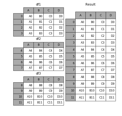
Figure1: Example from https://pandas.pydata.org/pandas-docs/stable/merging.html
For more information see http://pandas.pydata.org/pandas-docs/stable/merging.html.
Date and Time
Python can manipulate date and time objects using the datetime module. It allows the production of calculations using time and date objects and also provides classes for controlling the output (see also, https://docs.python.org/2/library/datetime.html)
from datetime import datetime
#%%
now = datetime.now()
now
and the result is
To get the date only
now.date()
and the output in this case is datetime.date(2017, 1, 6). To find the day
now.day
and the output is 6. Also, for the time
now.time()
and the output is datetime.time(14, 41, 4, 481168). We can also ask which is the week day:
now.weekday()
that will generate the output 4
from datetime import date, time
**
time(3, 24)
**
age = now - datetime(1980, 8, 16)
age/365
**
days=(datetime(2017, 3, 10) - datetime(2017, 8, 16))
days.days
Importing data
We suggest that you use comma-separated value or CSV files when interacting with Python and other statistical software. In computing, CSV files stores tabular data (numbers and text) in plain text. Columns are separated by commas; rows are terminated by newlines. This file format is not proprietary, the files can be edited in text editors and spreadsheet software, such as Excel and Calc.
dur = pd.read_csv("data/duration.csv", sep=";")
dur
Out[153]:
    experiment  duration
0            A       199
1            A       184
2            A       242
3            A       236
4            A       216
5            A       176
6            A       223
7            A       186
8            A       210
9            A       220
..         ...       ...
95           C       221
96           C       239
97           C       235
98           C       248
99           C       204
100          C       226
101          C       206
102          C       194
103          C       205
104          C       182

[105 rows x 2 columns]
We can also import another dataframe and add a column titled AA.
fricative = pd.read_table("data/fricatives.csv", sep=’,’)
fricative[’AA’] = pd.Series(range(1,8827))
**
fricative.head()
# %%
**
0   1  0.060398  32.671794   757.605236  1104.704765  13.835014  210.523631
1   2  0.045656  38.906220   732.582945  1065.089424  12.654465  186.856393
2   3  0.050907  47.209304   647.696728  1627.357767   7.647966   61.615315
3   4  0.051049  41.703970  1017.179353  2318.797907   5.570367   33.783925
4   5  0.028408  44.345609  1132.524942   848.894793   7.105495  108.453910

  Segment Vowel Variety      Stress   Voice Position   AA
0       d     a      CG  Unstressed  Voiced   Middle  1.0
1       d     a      CG  Unstressed  Voiced   Middle  2.0
2       d     a      CG  Unstressed  Voiced   Middle  3.0
3       d     a      CG  Unstressed  Voiced   Middle  4.0
4       d     a      CG  Unstressed  Voiced   Middle  5.0
**
list(range(1,len(fricative.index)))
We can skip rows if we do not want them in the analysis:
testfric=pd.read_csv("data/fricatives.csv", skiprows=[2,3,4,5,6])
len(testfric.index)
To import a small number of rows from, we can use nrows:
pd.read_csv("data/fricatives.csv", nrows=4)
**
get_ipython().system(’cat␣data/fricatives.csv’)
**
pd.read_csv("data/fricatives.csv").head(20)
**
pd.isnull(pd.read_csv("data/fricatives.csv")).head(20)
When we import data Python identifies empty cells, or NA values as NA data; to designated that specific values or symbols should be considered NA values, we can specify this as follows
pd.read_csv("data/fricatives.csv", na_values=[’?’, -9999999]).head(20)
Save Data
There are different methods to save data. To save data in CSV format
# ## Writing Data to Files
fricative.to_csv("fricative-01.csv")
Creating Plots
Using pandas we can also make some basic plotting.
fricative[’duration’].plot()
**
##############################################################
# %%
fricative = pd.read_csv("data/fricatives.csv", sep=’,’)
fricative[’duration’].plot()
# %%
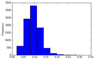
fricative[’duration’].plot(kind=’hist’)
# %%
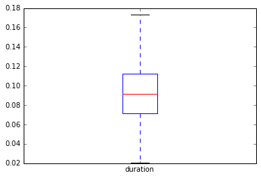
fricative[’duration’].plot(kind=’box’,showfliers=False)
Duration
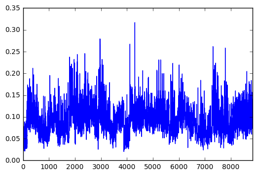 Figure2: Duration in sec.
 ————————————————————————
import matplotlib.pyplot as plt plt.plot([1,2,3,4]) plt.ylabel(’some numbers’) plt.show()
Basic Descriptive Statistics using Pandas
**
In [208]:

fricative.sum()
Out[208]:
duration                                               827.811
intensity                                               346024
cog                                                5.05981e+07
sdev                                               2.40776e+07
skew                                                   21699.9
kurt                                                    328392
Segment      dddddddddddddddddddddddddddddddddddddddddddddd...
Vowel        aaaaaaaaaaaaaaaaaaaaaaaaaaaaaaaaaaaaaaaaaaaaaa...
Variety      CGCGCGCGCGCGCGCGCGCGCGCGCGCGCGCGCGCGCGCGCGCGCG...
Stress       UnstressedUnstressedUnstressedUnstressedUnstre...
Voice        VoicedVoicedVoicedVoicedVoicedVoicedVoicedVoic...
Position     MiddleMiddleMiddleMiddleMiddleMiddleMiddleMidd...
AA                                                 3.89536e+07
dtype: object
**
In [209]:

fricative.mean()
Out[209]:
duration        0.093782
intensity      39.254023
cog          5732.200660
sdev         2727.724598
skew            2.458354
kurt           37.203150
AA           4413.500000
dtype: float64
**
In [211]:

fricative.std()
Out[211]:
duration        0.031759
intensity       8.272744
cog          3425.508087
sdev         1339.636724
skew            4.785687
kurt          138.622132
AA           2547.991071
dtype: float64
**
In [212]:

fricative.count()
Out[212]:
duration     8827
intensity    8815
cog          8827
sdev         8827
skew         8827
kurt         8827
Segment      8827
Vowel        8827
Variety      8827
Stress       8827
Voice        8827
Position     8827
AA           8826
dtype: int64
**
fricative.intensity.hasnans
Out[215]:
True
In [221]:

fricative.intensity.isnull().sum()
Out[221]:
12
Describe:
In [222]:

fricative.describe()
/Users/haristhemistocleous/anaconda3/lib/python3.5/site-packages/numpy/lib/function_base.py:3834: RuntimeWarning: Invalid value encountered in percentile
  RuntimeWarning)
Out[222]:
          duration    intensity           cog         sdev         skew  \
count  8827.000000  8815.000000   8827.000000  8827.000000  8827.000000
mean      0.093782    39.254023   5732.200660  2727.724598     2.458354
std       0.031759     8.272744   3425.508087  1339.636724     4.785687
min       0.020333     5.278827    419.757883   228.697624    -5.250996
25%       0.071596          NaN   2385.869561  1771.421219    -0.113557
50%       0.091452          NaN   6175.724355  2368.203536     0.925865
75%       0.112412          NaN   8344.008050  3595.757817     2.953676
max       0.316844    69.455969  18606.542539  9253.436646    59.853567

              kurt           AA
count  8827.000000  8826.000000
mean     37.203150  4413.500000
std     138.622132  2547.991071
min      -1.892874     1.000000
25%       0.512395          NaN
50%       3.432032          NaN
75%      12.453753          NaN
max    3999.613892  8826.000000
describe can detect non-numeric data and sometimes yield useful information about it.
**
fricative.sdev.describe()
Out[224]:
count    8827.000000
mean     2727.724598
std      1339.636724
min       228.697624
25%      1771.421219
50%      2368.203536
75%      3595.757817
max      9253.436646
Name: sdev, dtype: float64